3. Analyzing carbon allocation profile
3.1. Read dataframe with carbon allocation data
[29]:
# assume already have the flux snapshots at desired cycle
import os
import pandas as pd

import seaborn as sns
import matplotlib.pyplot as plt

from scarcc.preparation.find_directory import find_directory
from scarcc.data_analysis import get_fs_change
from scarcc.data_analysis import (get_row_color_legend, relabel_clustermap, generate_row_colors, assign_plot_total_E_wide,
                                    get_fs_kde_plot, plot_kde)


data_directory = find_directory('Data', os.path.abspath(''))
carbon_allocation_E_wide = pd.read_csv(os.path.join(data_directory, 'carbon_allocation_E_wide_checkerboard.csv'), index_col=0)
carbon_allocation_E_wide.query('XG=="DG"').head()
[29]:
| total_carbon_BIOMASS_Ec_iML1515_core_75p37M | total_carbon_EX_bulk_ac_e | total_carbon_EX_co2_e | total_carbon_EX_for_e | total_carbon_EX_glyclt_e | total_carbon_EX_hacolipa_e | total_carbon_EX_lcts_e | total_carbon_EX_met__L_e | total_carbon_Waste | percent_BIOMASS_Ec_iML1515_core_75p37M | ... | percent_Waste | XG | Drug_comb_effect_coc | Drug_comb_effect_Emono | Drug_comb_effect_Smono | BM_consortia_frac_binned | plot_total_carbon_Waste | plot_total_carbon_EX_bulk_ac_e | plot_total_carbon_BIOMASS_Ec_iML1515_core_75p37M | plot_total_carbon_EX_co2_e | |
|---|---|---|---|---|---|---|---|---|---|---|---|---|---|---|---|---|---|---|---|---|---|
| Gene_inhibition | |||||||||||||||||||||
| folP.folA_1.1 | -3.970327 | -4.657846 | -3.482788 | NaN | NaN | NaN | 12.509550 | 0.077759 | 0.398589 | -0.317384 | ... | -0.031863 | DG | Synergistic | Additive | Additive | E | 0.398589 | 4.657846 | 3.970327 | 3.482788 |
| folP.folA_1.2 | -2.786021 | -14.046874 | -4.051436 | -4.444467 | NaN | NaN | 47.013448 | 0.054564 | 21.684651 | -0.059260 | ... | -0.461244 | DG | Synergistic | Synergistic | Synergistic | S | 21.684651 | 14.046874 | 2.786021 | 4.051436 |
| folP.folA_1.3 | -1.354612 | -11.476818 | -5.213290 | -1.670134 | NaN | NaN | 42.266922 | 0.026530 | 22.552068 | -0.032049 | ... | -0.533563 | DG | Synergistic | Synergistic | Synergistic | S | 22.552068 | 11.476818 | 1.354612 | 5.213290 |
| folP.folA_1.4 | -0.151995 | -10.678128 | -5.035713 | -0.699630 | -1.895609 | NaN | 41.742689 | 0.002977 | 23.281615 | -0.003641 | ... | -0.557741 | DG | Synergistic | Synergistic | Synergistic | S | 23.281615 | 10.678128 | 0.151995 | 5.035713 |
| folP.folA_1.5 | -0.017016 | -10.593038 | -5.011159 | -0.595460 | -2.115722 | -0.000263 | 41.695097 | 0.000332 | 23.362439 | -0.000408 | ... | -0.560316 | DG | Additive | Synergistic | Additive | S | 23.362439 | 10.593038 | 0.017016 | 5.011159 |
5 rows × 27 columns
calculate the difference in secretion fluxes quantity, normalized carbon content in flux, between double drug addition and single drug addition
[30]:
gr_path = os.path.join(data_directory, 'gr_DG_checkerboard_normalized.csv')
fs_change = get_fs_change(gr_path=gr_path,carbon_allocation_E_wide=carbon_allocation_E_wide)
fs_change.head()
[30]:
| percent_BIOMASS_Ec_iML1515_core_75p37M | percent_EX_bulk_ac_e | percent_EX_co2_e | percent_EX_for_e | percent_EX_glyclt_e | percent_EX_hacolipa_e | percent_EX_lcts_e | percent_EX_met__L_e | percent_Waste | Nth_gene | Drug_comb_effect_coc | Drug_comb_effect_Emono | Drug_comb_effect_Smono | BM_consortia_frac_binned | plot_total_carbon_Waste | plot_total_carbon_EX_bulk_ac_e | plot_total_carbon_BIOMASS_Ec_iML1515_core_75p37M | plot_total_carbon_EX_co2_e | |
|---|---|---|---|---|---|---|---|---|---|---|---|---|---|---|---|---|---|---|
| Gene_inhibition | ||||||||||||||||||
| folP.folA_1.1 | -0.017740 | 0.016451 | 0.003070 | NaN | NaN | NaN | 0.0 | 0.000347 | -0.001781 | First | Synergistic | Additive | Additive | E | 0.398589 | 4.657846 | 3.970327 | 3.482788 |
| folP.folA_1.1 | -0.028156 | 0.005705 | 0.000058 | NaN | NaN | NaN | 0.0 | 0.000551 | 0.031863 | Second | Synergistic | Additive | Additive | E | 0.398589 | 4.657846 | 3.970327 | 3.482788 |
| folP.folA_1.2 | -0.268977 | -0.065494 | -0.189000 | NaN | NaN | NaN | 0.0 | 0.005268 | 0.428935 | First | Synergistic | Synergistic | Synergistic | S | 21.684651 | 14.046874 | 2.786021 | 4.051436 |
| folP.folA_1.2 | -0.275864 | -0.057108 | -0.189164 | NaN | NaN | NaN | 0.0 | 0.005403 | 0.427600 | Second | Synergistic | Synergistic | Synergistic | S | 21.684651 | 14.046874 | 2.786021 | 4.051436 |
| folP.folA_1.3 | -0.303075 | -0.084360 | -0.151998 | NaN | NaN | NaN | 0.0 | 0.005936 | 0.499919 | First | Synergistic | Synergistic | Synergistic | S | 22.552068 | 11.476818 | 1.354612 | 5.213290 |
subset of fs_change for passing into heatmap
[23]:
p_cols = ['percent_BIOMASS_Ec_iML1515_core_75p37M', 'percent_EX_bulk_ac_e', 'percent_EX_co2_e', 'percent_Waste']
total_carbon_cols = [ele.replace('percent', 'plot_total_carbon') for ele in p_cols]

response_cols = ['Drug_comb_effect_coc', 'Drug_comb_effect_Emono', 'Drug_comb_effect_Smono', 'BM_consortia_frac_binned']
p_cols_w_effect = p_cols + response_cols
fs_sub_change=  (fs_change
                .set_index('Nth_gene', append=True)
                .loc[:,p_cols_w_effect]).dropna(axis=0, how='any')

Normal_row = pd.DataFrame(0, columns = fs_sub_change.columns, index = ['Normal'])
Normal_row.loc[:,'Drug_comb_effect_coc':'BM_consortia_frac_binned']=None
Normal_row['Nth_gene'] = 'Normal'
Normal_row.index.name='Gene_inhibition'
Normal_row.set_index('Nth_gene', append=True, inplace=True)
Normal_row
fs_sub_change = pd.concat([fs_sub_change, Normal_row])
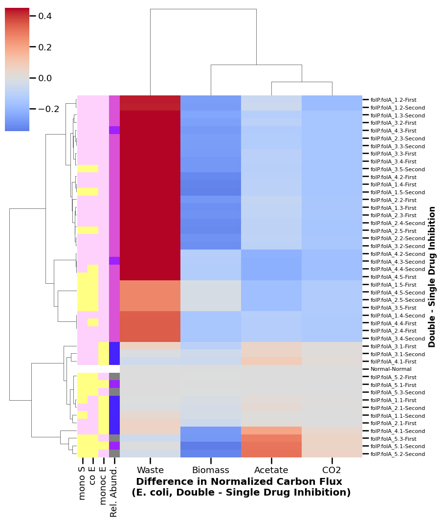
3.2. Heatmap
[24]:
sns.set_context('talk', font_scale=0.8)
fig = plt.figure()
clustered = sns.clustermap(fs_sub_change.loc[:,p_cols]
            , row_colors=generate_row_colors(fs_sub_change)
            # , standard_scale=1
            , center=0
            , yticklabels=True
            , figsize=(10, 14)
            , vmax=0.45
            , cmap='coolwarm')
relabel_clustermap(clustered)
['E', 'slight E', 'S', 'No growth']
<Figure size 640x480 with 0 Axes>
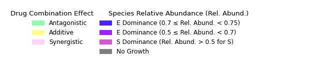
Add associated legend
[31]:
get_row_color_legend()
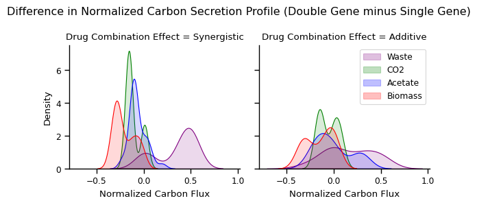
Kernel density estimation using normalized carbon flux data
[26]:
fs_plot = get_fs_kde_plot(fs_change)
plot_kde(fs_plot, col_prefix='percent_')
Index(['Drug Combination Effect', 'reaction', 'Normalized Carbon Flux'], dtype='object')
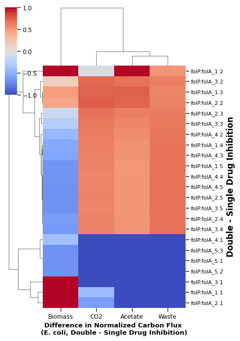
Heatmap of flux quantity per drug pair only
[ ]:
p_cols = ['percent_BIOMASS_Ec_iML1515_core_75p37M', 'percent_EX_bulk_ac_e', 'percent_EX_co2_e', 'percent_Waste']
total_carbon_cols = [ele.replace('percent', 'plot_total_carbon') for ele in p_cols]
sns.set_context('paper')

plot_cluster_disagree = assign_plot_total_E_wide(carbon_allocation_E_wide,log_waste=False).dropna(how='any')
row_colors = generate_row_colors(plot_cluster_disagree, color=[ '#4622fc','#9d22fc', '#da52d5', 'grey'])
clustered = sns.clustermap(plot_cluster_disagree[total_carbon_cols] # flux magnitude
            #    ,row_colors=row_colors
               , z_score=1
               , figsize=(5, 10)
               , vmin=-1, vmax=1
               , cmap='coolwarm')

relabel_clustermap(clustered)
['E', 'slight E', 'S', 'No growth']